ANN, CNN, FFN, RNN… That’s a lot of N’s! Even for someone ensconced in the field of neural networks, a subfield within machine learning, there is an overabundance of terms and it can be difficult to keep up. If you’re not in the data science field, and either want to break into it or think your business could benefit from implementing , then finding a starting point can be a challenge. I’ll try to make that task a little less daunting by explaining the three most common neural networks architectures you’ll encounter and utilize.
Feed Forward Network (FFN)
The FFN is the very first neural network you’ll see when learning about neural networks, with the iconic architecture shown in Fig.1. and discussed in my blog on demystifying neural networks.
 Fig.1. A feed forward network – every neuron in one layer passes information to every other neuron in the next layer.
The idea behind FFNs is relatively straightforward: each layer learns how to do something simple, and passes it to the next layer, with as few assumptions about the incoming data and as few restrictions on the network itself as possible. FFNs are, by far, the most general-purpose neural network, and are guaranteed to be able to give the correct answer given enough layers (each column of objects in Fig.1), enough neurons (those round things in Fig.1) in each layer, enough data, and enough time to train on the data. They also require a little luck – FFNs are pretty good at getting stuck in “local minima,” which are solutions that do a good enough job that the computer isn’t sure what the best way to make improvements is, but not good enough that we, as people, are satisfied. Here’s a pros and cons list of FFNs:
Pros
- They are general and easy tools.
- They are guaranteed to be able to solve the problem at hand (with constraints).
Cons
- Love and luck is needed – FFNs are certainly capable of solving the problem, but getting them to realize their full capability can be an enormous challenge.
- The size and shape of the data must be known and specified ahead of time – FFNs can’t handle surprises in the data.
- These things can get huge – if your input data is too big, you can’t hand all of it to a FFN all at once without either overloading your machine or waiting for approximately forever!
Convolutional Neural Network (CNN or ConvNet)
If I hand you a 4032×3024 resolution picture and ask you to identify what’s in it, I’m giving you 12,192,768 data points and asking you to classify them. That’s a lot of data, and that’s a big ask. Using a FFN in this scenario is absolutely not viable since there would be hundreds of millions of variables that must be compiled and optimized to categorize even just 10 different objects in the picture (see last Con under FFNs).
Convolutional neural networks were created to handle exactly these kinds of problems by learning to hierarchically identify small, patterned features contained within a larger dataset and aggregating and re-identifying features until the entire dataset has been examined.
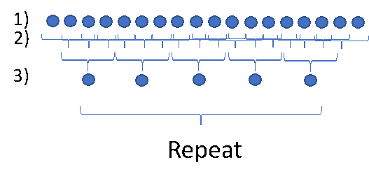
 Fig.2. A convolutional layer + pooling layer in a CNN.
Fig. 2 shows an example of a typical convolutional and pooling layer structure that executes precisely this feature-aggregating logic. Here, imagine the picture in the classification task above as a 1-dimensional line of data rather than a 2-dimensional set of pixels.
Row 1) is the set of input data that feeds into the CNN.
Row 2) examines every set of 3 consecutive input data points and applies the same logic to each of these sets. It’s like using a mini-FFN to learn the simpler task of identifying mini-features in the data rather than trying to classify it all at once. This is called the convolutional layer.
Row 3) identifies which of the overlapping chunks of data express specific features the strongest. For example, in an image, one chunk of data could contain part of a leaf, while the next one over contains the entire leaf. The network determines there is a leaf in some general area by taking the chunk in a region containing the full leaf as the representation for leaves. Another data chunk might contain a different feature that is not related to leaves. The process of keeping the champions of each feature in each segment of input data is called pooling, and the ‘layer’ that executes this logic is called the pooling layer.
The process of identifying the strongest features and aggregating is simply repeated until the entire dataset is appropriately classified.
Here’s a pros/cons list for CNNs:
Pros
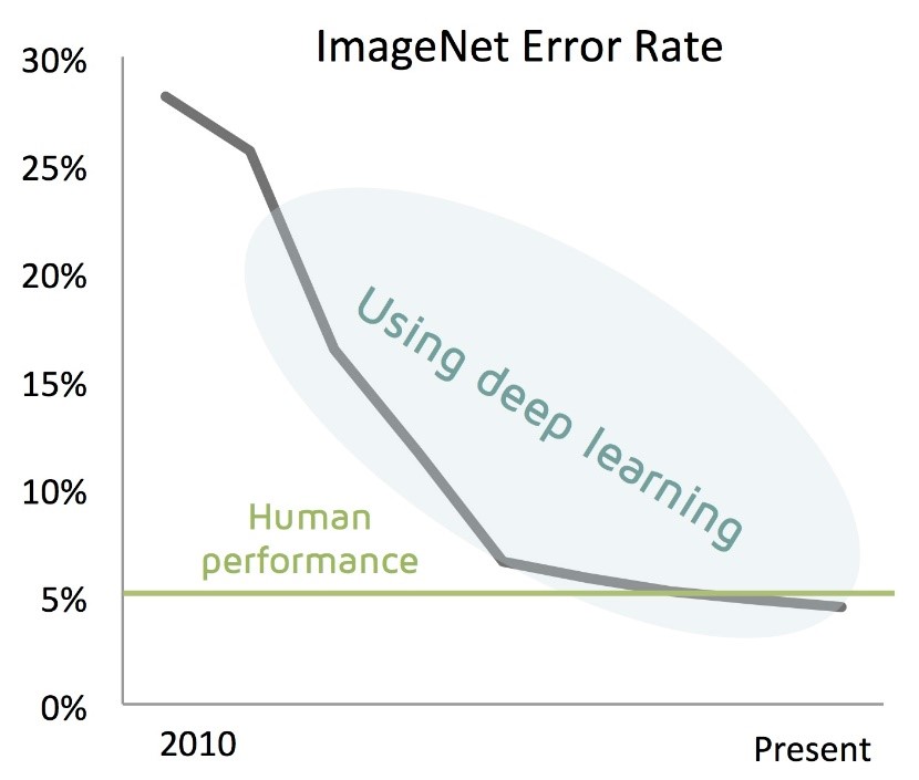
- Can identify patterns in 1D, 2D, …, N-D datasets exceedingly well. Indeed, CNNs outperform humans at image recognition now (see Fig.3).
- Require considerably fewer parameters than FFNs.
- Pooling is what’s called a ‘translation invariant’ operation. This just means it doesn’t matter where a pattern is in the data because it will still identify its presence.
 Fig.3. Deep learning now outperforms humans at classifying images.
Cons
- Requires a lot of data. They cannot generalize an example of a pattern, there must be enough data examples to confirm the pattern.. For instance, if the input data is text, words presented out of order will confuse it; for images, a network cannot identify an object in a picture if it is rotated relative to previous examples of that same object.
- The data doesn’t necessarily need to be a fixed size, but it certainly needs to be a minimum shape/dimension, and will struggle if the size of the data fed to it varies too wildly. While not as rigid as FFNs, CNNs share similar struggles with needing to specify the data size and shape.
Recurrent Neural Network (RNN)
CNNs are great at pattern recognition. Image recognition is an obvious application for such a network class, but, it turns out, natural language processing is another! We frequently speak and write by using patterns of words as templates, and gluing those patterns together. Idiomatic expressions are inherently patterns, as they frequently mean something different than their naive semantic interpretation. But, saying something in slightly different ways confuses a CNN. How, then, can we account for grammar and semantics when executing on natural language processing tasks?
Enter, recurrent neural networks. RNNs take a single, complicated function and apply it repeatedly to a sequence of data. The network keeps track of its understanding of the data it has read, and updates its understanding as new data is ingested with each application of the function it has learned. The architecture looks like Fig.4
 Fig.4. Each sequential data element (x’s) is read by the RNN (A) and outputs an updated understanding of the data (h’s). From Chris Olah’s blog on LSTMs.
RNNs excel at analyzing any series of data – stock prices through time, rainfall throughout the year, network activity, etc. In fact, they are unreasonably effective at these tasks. They are also generative. To this end, they are behind any deep learning-created piece of text, and modern approaches to language translation.
Of course, they, like all other networks, face obstacles. Here’s the pros/cons list:
Pros
- Unreasonably effective at ingesting (short) sequential data.
- The best act in town for generating (short) sequential data.
- RNNs learn one function very well and repeatedly apply it (no need to think too much about layers!).
Cons
- Memory loss. The single biggest challenge facing RNNs is how easily they lose information about old data. There are a few architectures that help mitigate this problem (gated recurrent units, or GRUs, and long short-term memory units, or LSTMs), but anything more than a few dozen data points will cause the network to begin forgetting the first ones it sees.
- RNNs are notoriously sensitive to how the model is ‘initialized’ – that is, how the model parameters that get optimized during training are first chosen. These issues have been largely overcome, but it’s still possible to see strange results with some bad luck.
Hopefully this overview has provided some useful insight into the most popular neural networks – both how they work, and when they’re useful. Interested in learning more? Contact us.